Advanced Radar Topics

Weather radar has come a long way since its early days of simply detecting precipitation. Today’s advanced radar forecasting techniques combine sophisticated technology with powerful algorithms to provide meteorologists with unprecedented insight into storm behavior and evolution. Let’s explore how these cutting-edge tools are transforming weather prediction.

Note from the author:

---

The content of this page is intended for educational purposes. While nearly all of the content comes directly from reputable sources (radar manufacturer manual, National Weather Service, my own collaboration with radar operators, etc), you should use this information at your own risk. Always have trustworthy & reliable sources for your weather alerts.

-Eric

---

Weather Radar

History of Radar

Early discoveries and experiments with “radar” date back to the late 19th Century although, at the time, it wasn’t called that.

While there’s some debate on the etymology , popular believe is that RADAR is actually a quassi-acronym, dating back to World War II. It’s believed the U.S. Navy coined the term, a shorter version of the name for the technology they used detecting/measuring distance of enemy ships/planes.

and so… RAdio Detection And Ranging became just… RADAR

Regardless of the origin of the word, the technology remains the same. Radar has many applications in our day-to-day lives, especially in weather awareness.

Discovering Weather Use

It’s possible weather radar was actually discovered somewhat by mistake. During this period in World War II, meteorologists noticed that precipitation created “noise” on radar screens. This discovery led to additional research and eventually the development of dedicated weather radar systems.

The specific type of Radar now used by NWS is the WSR-88D.

WSR-88D

The WSR-88D was developed in the late 1980’s and deployed for operational forecasting use in 1992 in Sterling, VA. Radars now operate in over 160 locations.

The WSR-88D radar operates on the S-Band of frequencies (2700-3000 MHz) and transmits pulses at 750,000 watts.

It can operate at many different angles of elevation (”tilts”). For example, the radar can go from 0° to 60° tilt above the horizon (but usually maxes out around 19.5° for operational use).

Things that can be seen on radar can be moisture (rain/ice), birds/insects, debris, wind turbines, and airplanes.

---

So, before anyone gets all squirrelly about the effects of radiation from weather radar… they might want to consider all the other things people put by their beds, into their pockets, in their ears, etc.

---

The WSR-88D is a fabulous tools, and like with any tool, it comes with strengths and limitations.

Weather Radar Principles

Radar operates by sending out a pulse of radio wave. If that radio wave encounters something in its path, it will reflect a radio wave back to the radar.

Radar Terms

Here is a list of basic radar terms:

• Doppler - type of radar used for monitoring weather
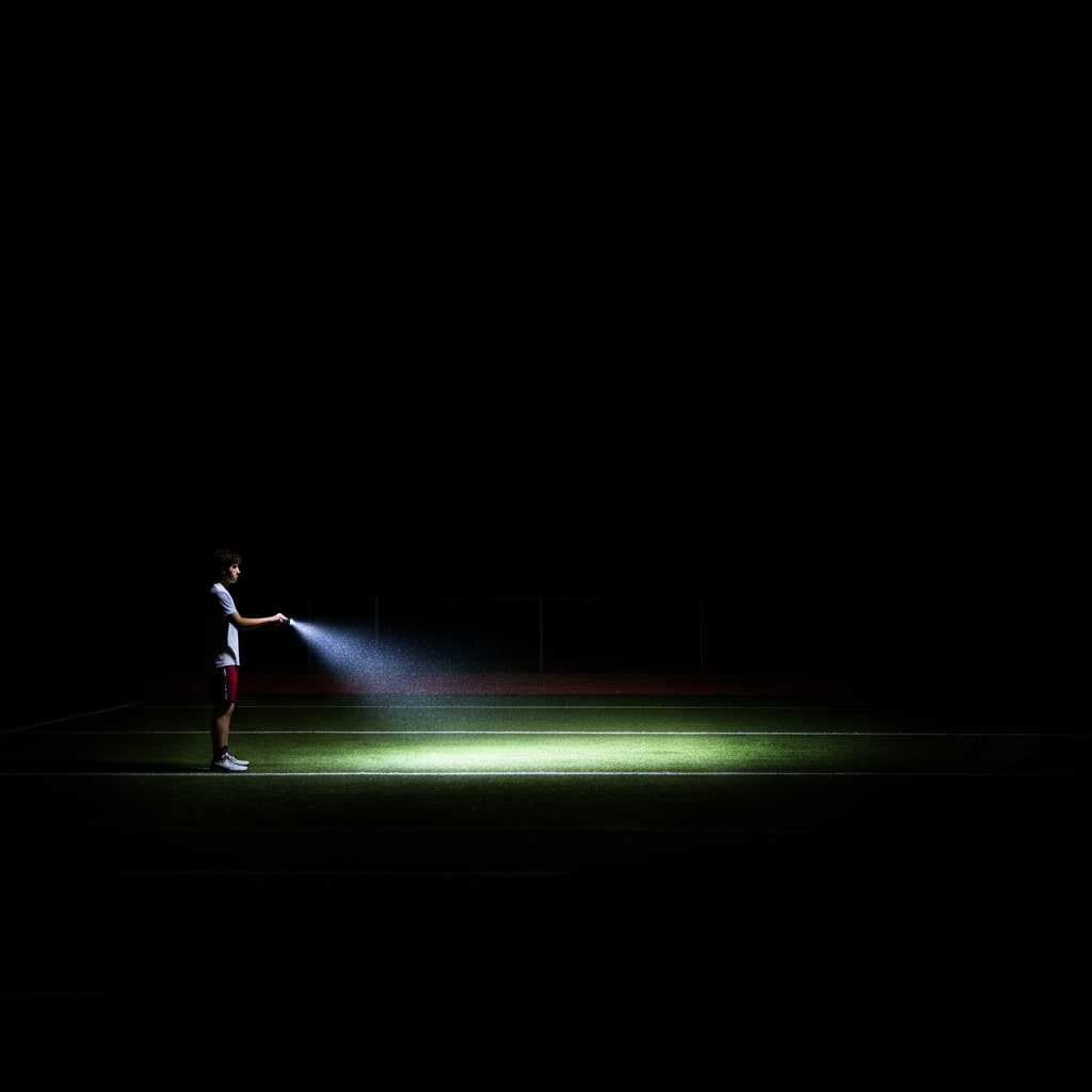
• Beam - describes the signal of the radar, similar to light from a flashlight
  
• Tilt - describes the angle of elevation the radar is sending/receiving it’s signals at. Each rotation of the radar scans at a specific tilt.
  
• Volume Scan - Multiple rotations/tilts are used to survey different parts of the atmosphere. Collectively they make up a volume scan.
  
• Echo - name for the reflected signal back to the radar. The characteristics of the Echo determines the size/shape/density/movement of the object.
  
• Radial - the angle or degree of the beam, left/right relative, to center. The radar completes a full 360-degree rotation, analyzing the atmosphere in all directions.
  

Beam Characteristics

When the beam leaves the radar, it travels away in a straight line. However, two very important characteristics impact the actual path of the bream.

Beam Size Over Distance

A radar beam expands dramatically as it travels through the atmosphere, spreading approximately 1,000 feet for every 10 miles it travels. That means, at 60 miles from the radar site, the beam has widened to about 6,000 feet (over a mile).

A radar beam acts similar to the beam of a flashlight. The farther away the beam gets from the flashlight (radar), the wider the area of coverage will be.

This initially sounds good…but, consider this analogy:

This is very similar to what happens with radar: the further away an object is, the weaker returns and less detailed information is returned.

Impact of Earth Curvature

As a radar beam travels away from the radar, it increases slightly in elevation. At long distances, radar can actually overshoot objects and miss them altogether. This is partially due to Earth’s curvature and partially due to other physical phenomena in our atmosphere.

Put simply, as the beam travels away from the radar, the Earth curves down and away, leaving the beam appearing to increase in elevation.

The beam’s path is partially impacted by atmospheric refraction .

Atmospheric refraction can further bend the beam upwards or even bend it down towards Earth. It’s different every day!

However, on average, this refraction results in a net curvature that is slightly less than the Earth’s (i.e. so basically: slightly up in elevation) - see the image below.

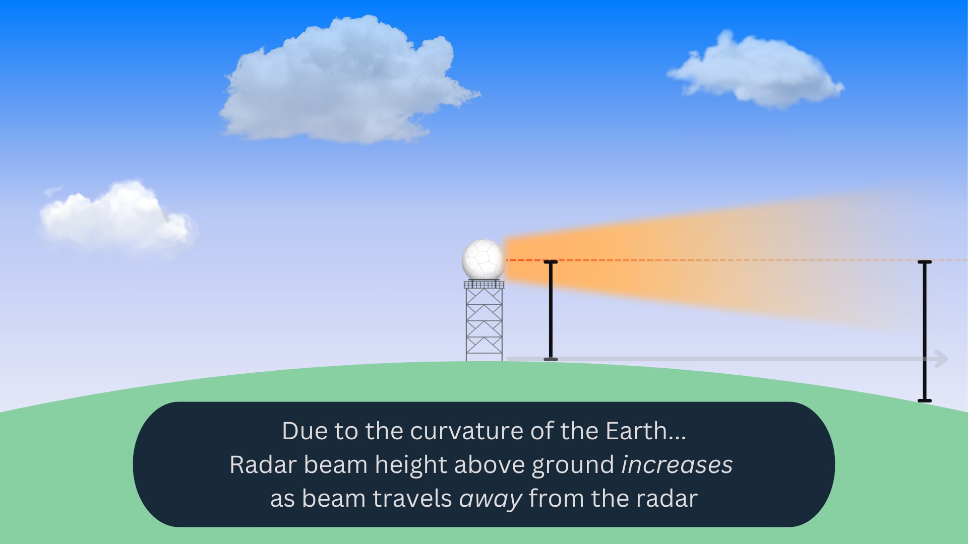
The key take away is that radar will struggle to “see” objects near the ground at long distances.

Doppler Radar

Doppler Radar is a unique type of radar that analyzes objects using the Doppler effect .

It is the type of radar used by most weather operations, including the National Weather Service (NWS). Its technology is what allows the measurement of things like wind speed and rotation, in addition to the detection and analysis of rain.

Radar analyzes the atmosphere by sending electromagnetic pulses of energy out and receiving an “echo” (response) back.

The amplitude of the echo signal and time it takes to get back to the radar, determines the type/density of object and how far it is away.

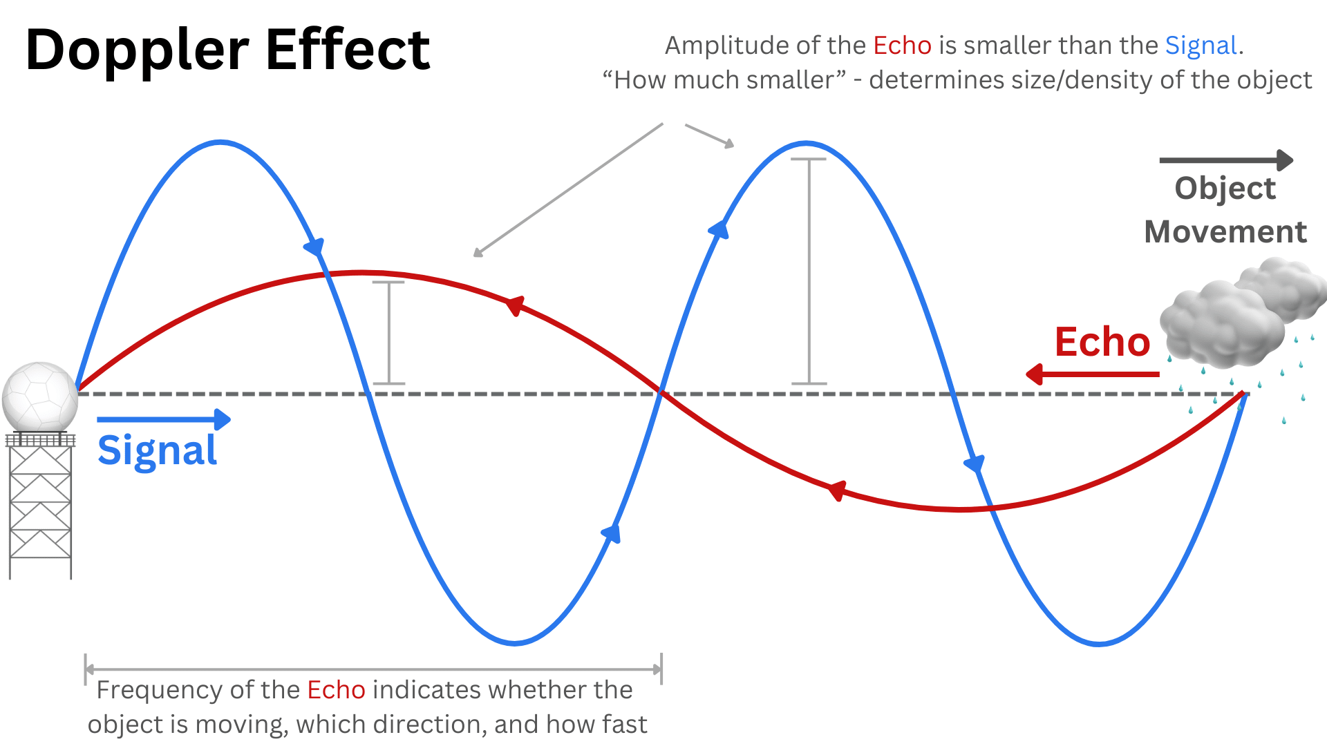
If the object is stationary, the echo signal will be a mirror of the transmission. If the object is moving, the frequency of the echo will change. The magnitude of this change determines how fast the object is moving and what direction.

Here’s a conceptual image showing a radar signal and associated alteration of an Echo (response). Notice the blue signal leaving and the red echo returning have different amplitudes and frequencies.

Radial Velocity

A topic discussed briefly on the Radar Basics page is that Doppler radar can only measure Radial Velocity . Radial Velocity is such an important topic, it’s getting it’s own sub-section here.

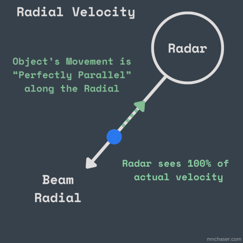
Radial Velocity refers to a Doppler radars ability (or limitation in this case) that it can only measure the speed of an object traveling directly along (parallel to) the beam (“radial”). See conceptual “perfect” scenario below.

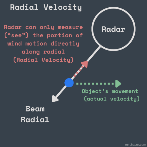
This also means, if an object is moving perfectly perpendicular (sideways) to the radar radial, the radar will calculate a velocity of 0!

More realistically, objects will be moving at some angle relative to the radial. In these cases, the radar will only be detecting the portion of motion that is directly along the radial - which will always be less than the actual velocity.

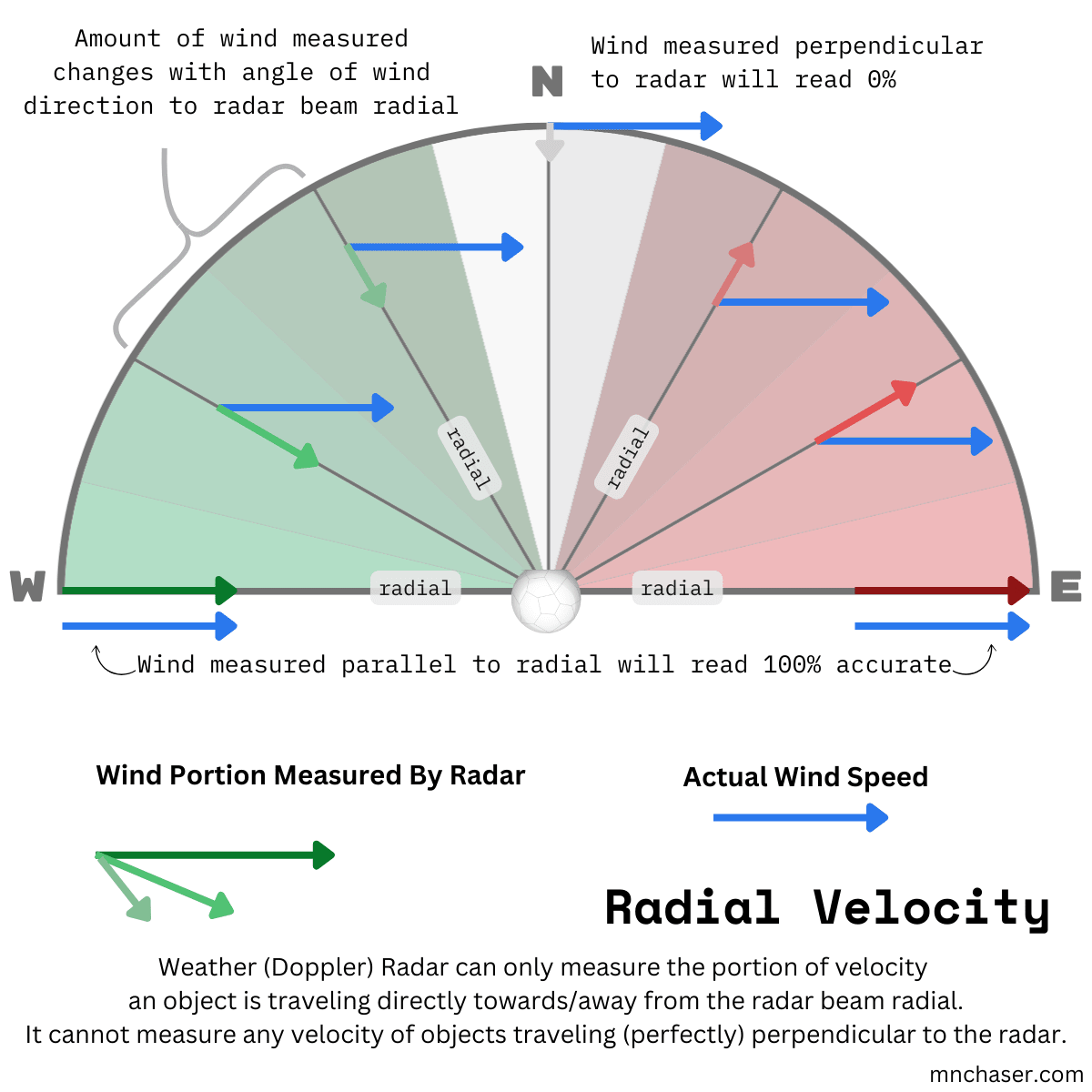
Here’s another image which applies radial velocity to half of a velocity scan.

Estimating actual wind speed

Estimating actual wind speed is a complex topic involving trigonometry . Plus, you need to be confident in the direction wind is moving in order to calculate the angle relative to radial.

You can make some crude estimates to the actual velocity, by following these steps:

1. At a particular location, find the Radial Velocity and estimated direction of wind
2. From that location, draw a straight line back to the radar (this is the radial)
3. Estimate the angle of the wind direction to the radial, using hours on a clock as a guide
4. Use the list below to estimate the actual wind velocity

Here’s a more accurate look at those values and the corresponding % wind component:

• 12:00 - 0° - 100%
• 1:00 - 30° - 87%
• 2:00 - 60° - 50%
• 3:00 - 90° - 0%
• 4:00 - 120° - 50% (same as 60°)
• 5:00 - 150° - 87% (same as 30°)
• 6:00 - 180° - 100% (same as 0°)

As you can see, there is a pretty sharp

Practical Example

Bringing all these considerations together, look at the image below. It is a more accurate, conceptualized view of how wind/velocity data often looks.

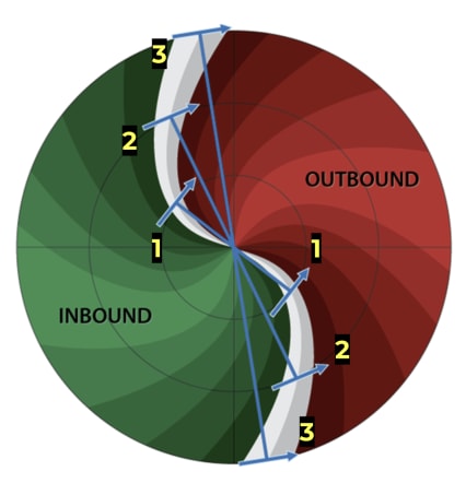
Notice the “S” shape of the radar. This is a very common pattern we see in the Northern Hemisphere.

1. At the radar site (center) and along line 1, we can see surface winds SW -> NE
   
2. Moving away from the radar towards arrows #2, winds take on a more W,SW -> E,NE direction
   
3. Near arrows #3, the outer edge of our scan, we can see winds are taking almost a W -> E path
   

Notice, as you move away from the center, the direction of the wind change is uniform above and below the radar. Not only does this present north and south of the radar, but these locations are higher in altitude than the center, due to the increased beam height.

From this analysis, one can determine broad wind shear occurring, with change in wind direction SW to W with elevation!

Radar Summary

Volume Coverage Patterns

algorithm used by radar

Volume Coverage Patterns (VCPs) are like mode that can configure how a radar scans, depending on what type of conditions are present. There are two main groups of VCPs:

Clean Air Mode - This mode is characterized by slower antenna rotation rates, which allows the radar to sample the atmosphere for longer periods.

Precipitation Mode - This mode operates with faster antenna rotation rates to effectively track active weather systems.

A VCP tells the radar what speed and what angles (tilts) to use for each revolution. Once all tilts have been measured, the volume scan is considered complete. Radar operators, and intelligence programmed into the radar itself, make key decisions in the trade-off between which elevations, time, and quality based on conditions.

The number of patterns has simplified over time, so we’ll focus on the major ones you will likely see.

Clear Air Mode

The slower rotation of Clear Air Mode enables finer resolution and increased sensitivity, making it possible to detect subtle atmospheric conditions even when there’s no precipitation.

You’ll likely see one of these patterns during Clear Air mode.

VCP 35 - Default

• 9 elevation tilts in 7 minutes
• default mode
• used when no precipitation or very light drizzle is expected

VCP 31 - Winter

• 5 elevation tilts in 10 minutes
• uses a longer pulse length
• helpful in the winter, detect snow or freezing moisture (despite clear air)

Precipitation Mode

When precip or storms are expected, radar operators may switch the radar into Precipitation Mode. Radars can also configured to also automatically switch to Precip Mode, if rain is detected by the radar.

Precipitation Mode is specifically designed to monitor and track precipitation events, including rain, snow, and thunderstorms. The faster scanning (rotation) can track rapidly changing weather conditions and provides us more frequent updates during severe weather events.

VCP Storm Patterns

Two common patterns used during inland severe weather are VCP 12 and VCP 212. The primary difference between them is VCP 212’s enhanced algorithms for solving problems with range folding.

VCP 12 - Default

• 14 tilts in 4.5 - 5 minutes
• fastest scan
• basic range folding algorithm
• if default algorithm can not resolve, velocity data is lost

VCP 212 - Storm

• 14 tilts in 4.5 – 5 minutes
• advanced algorithm for range folding problems
• requires specific radar configuration
• greatly improves velocity values
• additional ~30s run time over VCP 12

During tropical storms, even the advanced algorithm in VCP 212 is not sufficient enough to provide the fidelity of data needed to monitor hurricane velocities. VCP 112 was created to solve for this unique challenge. It sacrifices some additional run time for additional processing to calculate more precise velocity values.

VCP 112 - Tropical Storm

• 14 tilts in 5.5 minutes
• uses multiple algorithms and additional techniques to improve velocity values
• this is helpful for tropical cyclones (hurricanes)
• extra scan time is acceptable for the tradeoff benefit

VCP Surveillance Patterns

For general widespread, non-severe precipitiation monitoring, a common pattern used is VCP 215.

VCP 215 - Non-Storm

• 15 tilts in 6 minutes
• general surveillance pattern
• better quality data for widespread precip events without storms
• too slow for rapidly developing thunderstorms

Dual Polarization

Early weather radar systems could only emit radio waves using a single wave.

For the Base Products (Reflectivity, Velocity, Spectrum Width), single polarization ) is sufficient for producing quality results.

However, the problem With this configuration, the radio waves could detect something, estimate it’s density, but had difficulty estimating its shape.

With Single Polarization, it is difficult to tell the shape of the objects detected. Is it a wide rain drop? or a circular hailstone? To Single Polarization, they look very similar.

As technology advanced, Dual Polarization (Dual-Pol) radar was introduced - using both horizontal and vertical orientations simultaneously.

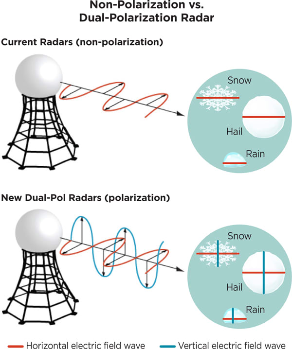
The advanced technology in Dual Polarization offers a host of new products and capabilities based on shape.

Dual Polarization radar can:

• distinguish between different types of precipitation (rain, snow, hail)
• detect non-meteorological objects like birds, insects, and tornado debris

This capability dramatically improves forecasting accuracy and provides crucial information during severe weather events.

Dual Polarization Products

The following are a list of Dual-Pol products and benefits:

• Differential Reflectivity - measures how circular objects are
• Correlation Coefficient - measures how similar an object is to surrounding objects
• Specific Differential Phase - measures

A LOT more on Dual Polarization products can be found on the Radar Techniques page.

Challenges with Radar

Several challenges exist with radar, primarily driven by limitations or side effects of physics.

Range Folding

pulses and echoes are out of sync

Range Folding is a phenomenon where some of the response data (echoes) return to the radar AFTER the next pulse has already been sent.

When this occurs, the radar cannot determine which pulse the echo is returning from making it very difficult to interpret data, specifically velocity data .

Algorithms

One of the techniques to solve for range folding is to leverage advanced algorithms to process the response data. These algorithms can help “re-calculate” some of the velocity values that would otherwise be lost.

Range Folding can occur with Reflectivity data too! However, it would not be acceptable to have missing chunks of information on the Reflectivity products when monitoring severe weather!

So, algorithms alone are not the best overall solution.A better solution to solve for Range Folding for Velocity AND Reflectivity is to configure the radar to do Split Cut Scans .

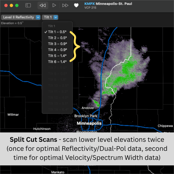
Split-Cut Scans

Double scans at each angle

Radar “Tilts” are actually nothing more than “slots” in a VCP algorithm: they can be configured to operate at different angles and collect different types of data for that scan.

With Split-Cut Scans, during the lowest elevations (typically 0.5°, 0.9°, and 1.3°) the radar is configured to scan each of these angles twice .

---

In the lower levels, split-cut scans use up an extra tilt (slot) for each angle, but the trade-off is worth it.

---

1. The first scan uses a faster pulse (to get a quicker response). This scan is used to collect Reflectivity and Dual-Pol data, at the sacrifice of poor Velocity data.
2. The second scan runs at the same tilt, but uses a slower pulse. The slower pulse provides much higher quality Doppler data (which calculates Velocity and Spectrum Width) at a sacrifice to Reflectivity quality and limited distance. Algorithms can typically resolve most Range Folding issues for this data.

Depending on the radar application and data available to you, you may be able to see the full list (or just a subset) of the tilts configured in a full volume scan.

In the image below, notice, Tilts 1 & 2, 3 & 4, and 7 & 8 are all the share the same angle.

Full Volume Scan Duration

As discussed under Volume Scan Patterns (VPCs) , typical VCP algorithms take approximately 5 minutes to complete.

Imagine this scenario:

Storms are developing rapidly…

• The risk of a mesocyclone, or even a tornado, is top of mind
• Radar is providing critical information about reflectivity and velocity near the ground
• You are monitoring values in the lowest elevations (especially 0.5°) for signs of rotation

Now, imagine waiting 5 minutes! for a full scan to complete, just to get an update on valuable 0.5° data!

That sort of delay would be massively detrimental when it comes to providing advanced warning of dangers with severe weather. A Solution? Yes! SAILS

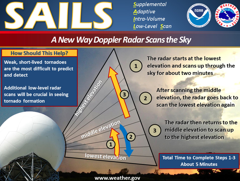
SAILS

Supplemental Adaptive Intra-Volume Low Level Scan (SAILS) – is a VCP configuration algorithm that enables the lowest elevations to be scanned more frequently, during severe weather events.

Not to be confused with Split Cut Scans , the purpose of SAILS is to increase the frequency in which certain elevations are scanned. Instead of waiting a full 5 minutes to restart a scan, lower levels are scanned multiple times through a full volume scan.

This may seem inefficient at first, but with SAILS, low-levels can be scanned every 1.8-2.5 minutes - more than twice as fast as a full scan.

SAILS patterns are configurable too. Radar operators can choose to run 1, 2, or 3 additional “SAILS” scans.

Here is an example of a VCP 212 w/ SAILSx2 profile:

Tilt 1: 0.5° (Reflectivity) - 0.5° (Velocity) (Split Cut)
Tilt 2: 0.9° (Reflectivity) - 0.9° (Velocity) (Split Cut)
Tilt 3: 1.3° (Reflectivity) - 1.3° (Velocity) (Split Cut)
Tilt 4: 1.8° (Reflectivity/Velocity)
Tilt 5: 0.5° (Reflectivity) - 0.5° (Velocity)
Tilt 6: 2.4°
Tilt 7: 3.1°
Tilt 8: 4.0°
Tilt 9: 5.1°
Tilt 10: 6.4°
Tilt 11: 0.5° (Reflectivity) - 0.5° (Velocity)
Tilt 12: 8.0°
Tilt 13: 10.0°
Tilt 14: 12.5°
Tilt 15: 15.6°
Tilt 16x: 19.5°

in this configuration, 0.5° is scanned every ~108 seconds.

Impact of SAILS

Here is a table showing the benefit of running a SAILS profile.

	Full Volume Information		0.5° Information
	Scan Frequency (sec)	Scans Per Hour	Scan Frequency (sec)	Scans Per Hour
VCP 212	every 243s	14	every 243s	14
VCP 212 (with SAILS)	every 305s	11	avg. every 108s	33

With SAILS, because 0.5° is scanned more frequently…

• time for a full volume scan increases , albeit only very slightly
• number of 0.5° scans per hour more than doubles !

This is a HUGE gain!

New technology exists now to interpret data coming back from each scan and adjust the number of supplemental SAILS scans and placement within the full range scan. So, depending on the situation, your radar may be operating slightly differently - and changing periodically.

Conclusion

Advanced radar forecasting techniques have revolutionized meteorology, providing unprecedented insight into storm structure and evolution. From Dual Polarization technology to machine learning algorithms, these tools help weather experts issue more accurate and timely warnings, potentially saving lives during severe weather events.

Additional Reading

The influence of scanning strategies on observations

Great read if you are into the impact/benefits SAILS has had on things like Thunderstorm Warnings and Tornado Warnings.